All source files — kernels, benchmarks, analysis scripts, and gem5 config — are in the github repository.
Goal
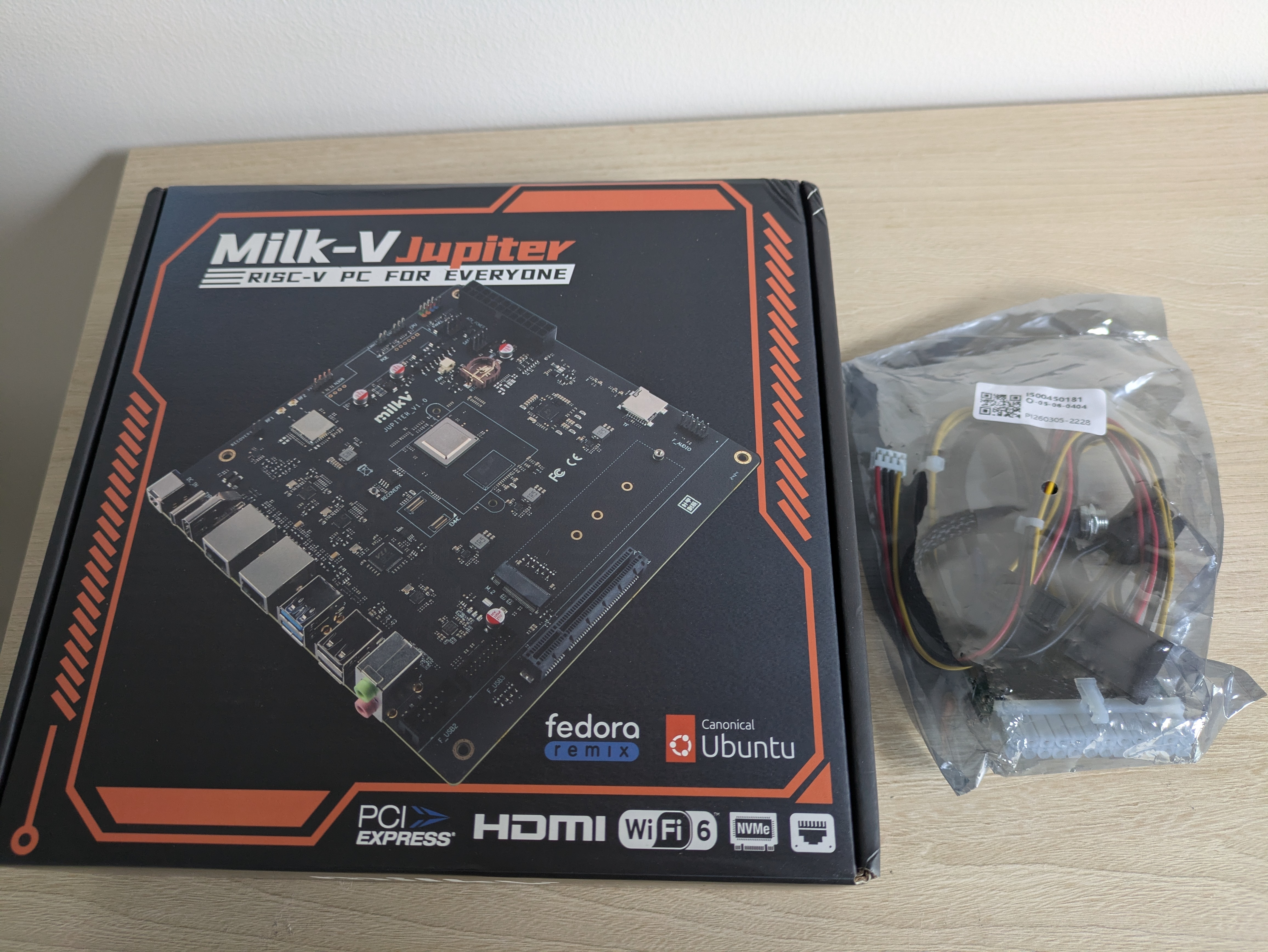
Liquid AI’s LFM2 class of foundation models are designed for fast on-device inference. As I await delivery of a Milk-V Jupiter RISC-V board to deploy these models on, I wanted to understand the current state of RVV vectorisation in llama.cpp for the LFM2 models — and whether there was a meaningful improvement to be gained in simulated performance.
Finding the gap
LFM2’s hybrid architecture interleaves 10 Linear Input-Varying (LIV) short convolution blocks with 6 GQA attention blocks. The technical report is available here.
Each layer routes through either a shortconv block or an attention block. The GQA blocks use grouped-query attention with RoPE and per-head QK normalisation. The shortconv blocks are the focus of this analysis assuming the RISC-V RVV paths don’t exist yet in llama.cpp.
What the shortconv block actually does. Inspecting build_shortconv_block in
src/models/lfm2.cpp shows the full compute graph which implements Section 2.2 of the technical report:
cur  →  in_proj  →  [b, c, x]
bx   =  b × x
bx   =  concat(conv_state, bx)
conv_out = ggml_ssm_conv(bx, conv_kernel)
y    =  c × conv_out
out  →  out_proj back to hidden_size
The single projection in_proj maps d_model → 3 × d_model, producing three equal chunks b (input gate), c (output gate), and x (input signal) via non-allocating views into the projected output. For LFM2-700M, d_model = 1536, so this is a 1536 → 4608 projection.
The product bx = b × x makes the convolution input data-dependent — the effective signal entering the filter varies with the current input, which is the “Linear Input-Varying” property. c is held as a multiplicative gate applied after the convolution: y = c × conv_out.
ggml_ssm_conv is used in LFM2’s shortconv blocks as a standalone depthwise 1D convolution. The conv state buffer holds d_conv - 1 historical columns per sequence giving a 4-tap filter: keeping the convolution causally correct across chunk boundaries.
Inspecting the ggml source confirmed that ggml_ssm_conv, implemented in
ggml_compute_forward_ssm_conv_f32, has no RVV fast path — it falls back to a plain
scalar C loop on all RISC-V targets. This will be the focus of the rest of this post.
What the ssm_conv kernel computes
The kernel performs a depthwise 1D convolution: each of the d_inner = 1536 channels has
its own independent 4-tap filter, with no mixing across channels. The convolution operates at the full model dimension with no separate expansion i.e. d_inner = d_model.
The key dimensions are:
| Symbol | Variable | Value |
|---|---|---|
d_inner | nr | 1536 |
d_conv (filter width) | nc | 4 |
n_t | tokens per sequence | T |
n_s | sequences in batch | B |
The padded input buffer conv_x has shape [d_model, d_conv - 1 + T]
where rows are channels (d_model = 1536) and columns are the sequence
positions (ncs = d_conv - 1 + T). The first d_conv - 1 = 3 columns
are the conv state — the 3 history values written back by the previous
token step. For each channel row and token position t:
output[d, t] = sum_{k=0}^{3} conv_x[d, t+k] * weight[d, k]The scalar implementation is four nested loops — sequences, tokens, d_inner rows, and
d_conv taps:
for (int i3 = 0; i3 < n_s; ++i3) {
  for (int i2 = 0; i2 < n_t; ++i2) {
    for (int i1 = 0; i1 < ir; ++i1) {       // d_inner rows (thread slice)
      float sumf = 0.0f;
      for (int i0 = 0; i0 < nc; ++i0) {     // 4 taps
        sumf += s[i0 + i1*ncs] * c[i0 + i1*nc];
      }
      x[i1] = sumf;
    }
  }
}
The widget below shows how the destination matrix is computed across the channel and token
dimensions. As the window slides across src0 per row, the same four convolution weights
in src1 are used to accumulate the result in dst.
RVV and memory layout
The data arriving at ggml_ssm_conv is the result of a fixed sequence of ggml graph operations in lfm2.cpp:
ggml_transpose()      ← makes d_model the slow axis (ne[1])
└── ggml_concat() ← prepends the rolling conv state along ne[0]
└── ggml_ssm_conv() ← receives nb[1] = ncs × sizeof(float) bytes
between adjacent channel rows
The transpose is required by the concat — the rolling conv state must be prepended along the sequence dimension, and the concat expects the sequence dimension to be the fast axis. The concat is required for correctness — it is how the sliding window of past token states is maintained across generation steps.
The consequence is that ggml_ssm_conv structurally receives a layout where
the channel dimension (d_inner = 1536) is the slow axis, with a stride of
ncs × 4 bytes between adjacent channels. For a 64-token prefill,
ncs = 67 and the inter-channel stride is 268 bytes. Vectorising across
channels — the natural strategy for RVV given conv_dim = 1536 — requires
loading elements separated by 268 bytes. Later sections explore how this can be achieved using both vector and scalar approaches.
Why the naive RVV approach is inefficient
An obvious choice would be to vectorise the innermost d_conv dot product — load 4 floats,
multiply, reduce to a scalar. A 4-element reduction requires a horizontal vfredusum, which is a
serial dependency chain that partially serialises the pipeline. For four scalar multiplies we will pay the full vector overhead and the reduction length will fit in a single register
group - not making full use of RVV’s 32 registers.
The proposed kernels are available here.
RVV v1 - An improved strategy: vectorise across d_inner rows
A better axis may be d_inner. Compute vl rows simultaneously — each vector lane owns one
complete channel to accumulate the sliding convolutions. For tap k across vl rows:
vsum[0..vl-1] += conv_x_col_k[0..vl-1] * weight_col_k[0..vl-1]With d_conv = 4 taps the full dot product for all vl rows collapses to
14 vector instructions: one vfmv_v_f to zero the accumulator, then for
each of the 4 taps two vlse32 loads and one vfmacc, and finally one
vse32 — versus vl × 4 scalar multiply-accumulate instructions for the
equivalent scalar code.
while (rows_left > 0) {
    size_t vl = __riscv_vsetvl_e32m4(rows_left);
    vfloat32m4_t vsum = __riscv_vfmv_v_f_f32m4(0.0f, vl);
    for (int i0 = 0; i0 < nc; ++i0) {
        vfloat32m4_t vs = __riscv_vlse32_v_f32m4(
            s + i0 + i1*ncs, ncs * sizeof(float), vl);
        vfloat32m4_t vc = __riscv_vlse32_v_f32m4(
            c + i0 + i1*nc,  nc  * sizeof(float), vl);
        vsum = __riscv_vfmacc_vv_f32m4(vsum, vs, vc, vl);
    }
    __riscv_vse32_v_f32m4(x + i1, vsum, vl);
    i1 += vl; rows_left -= vl;
}
Similar to the QWEN-2.5=0.5B post here, LMUL=4 at 256-bit VLEN gives vl = 256/32 * 4 = 32 lanes maximum. So each iteration of the while loop processes up to 32 channel rows simultaneously, and for d_model=1536 the loop runs ceil(1536/32) = 48 iterations. The total instruction count for one complete token step is therefore:
48 iterations × 14 instructions = 672 vector instructions
vs.
1536 channels × 4 instructions = 6144 scalar instruction
The widget below demonstrates the v2 approach using reduced dimensions:
RVV v2 - Strided memory access and the transpose problem
The vlse32 instruction gathers one element per row across vl rows using a fixed
stride. The stride between consecutive rows of conv_x is ncs × sizeof(float) bytes,
where ncs = d_conv - 1 + n_t. At n_t=4, ncs=7 and the stride is 28 bytes — under a typical cache line. At larger sequence lengths the stride grows and each gathered element
lands on a distinct cache line, potentially turning a single vlse32 into 32 independent cache miss
requests.
The v2 kernel attempted to eliminate this by transposing conv_x into a contiguous
temporary buffer before the MAC loop, replacing vlse32 with unit-stride vle32. The
problem is that the transpose is itself a strided read — the same access pattern as
vlse32 — paid in full as a pre-pass before any vectorised arithmetic begins.
RVV v3 — scalar gather with unrolled vector MAC
V3 takes a different approach to the strided access problem. Rather than using vlse32 to
gather tap columns directly into vector registers — which issues vl simultaneous cache
line requests — v3 uses a scalar loop to pack each tap into a contiguous temporary buffer
first, then loads those buffers with unit-stride vle32.
gem5 results — TimingSimpleCPU, D_INNER=1536
| n_t | Scalar | RVV v1 | RVV v2 | RVV v3 | v1 vs scalar |
|---|---|---|---|---|---|
| 4 | 833,632 | 1,014,995 | 1,533,561 | 1,203,277 | +21.8% slower |
| 16 | 1,183,248 | 2,735,712 | 6,404,849 | 3,554,770 | +131% slower |
| 64 | 2,942,876 | 8,397,648 | 23,694,856 | 11,695,748 | +185% slower |
| 512 | 15,087,584 | 82,341,980 | 197,887,936 | 106,526,045 | +446% slower |
**Cycles comparison across n_t values
Key finding: scalar wins at all token counts! The penalty worsens with token count because ncs = d_conv - 1 + n_t grows with n_t, increasing the vlse32 stride and the total L1D
access volume. At n_t=512 RVV v1 generates 16× more L1D accesses than scalar, with IPC collapsing to 0.104 versus scalar’s 0.436.
Why scalar still wins. The scalar kernel accesses conv_x sequentially: four
consecutive floats per row, then the next row — a monotonically-increasing stream the
prefetcher would follow easily.
Next steps: Milk-V Jupiter deployment
The simulation results establish a clear hypothesis — scalar outperforms all
three RVV kernel variants for ggml_ssm_conv across every tested token
count, with the penalty growing from +21.8% at n_t=4 to +446% at
n_t=512. Physical validation on the Milk-V Jupiter is the necessary next
step before drawing conclusions about real deployment performance.
The Jupiter’s SpacemiT X60 differs from the gem5 model in a number of ways that will impact these results. First, the real hardware prefetchers may partially hide the
strided load latency in ways that TimingSimpleCPU cannot model — the X60 could track the ncs-stride access pattern in the scalar kernel and begin issuing speculative fetches. Second, the real LPDDR4X memory subsystem has different latency and bandwidth characteristics than the LPDDR3-1600 model used in the simulation.
Running a full llama-bench comparison with and without the
ggml_ssm_conv RVV kernel against LFM2-700M-Q4_K_M.gguf will quantify
the end-to-end impact on prefill and decode throughput — key metrics that
matter for practical edge deployment.
Oh. Look what just arrived..